Useful Data Structures

• Hashing
  • Basic Concepts
  • Performances
• 1. Bloom Filter
  • 1.1 Algorithmic Description
  • 1.2 False Positive Analysis

Hashing

Basic Concepts

Definition 1: [Simple Uniform Hashing] A randomized algorithm $H$ for constructing hash functions $h: U \rightarrow \{1,...,M\}$ is called as simple uniform hashing, if given any element is $U$ is equally likely to hash into any of the $M$ slots.

Definition 1: [Universal Hashing] A randomized algorithm $H$ for constructing hash functions $h: U \rightarrow \{1,...,M\}$ is called universal, if for any $x \neq y$ in $U$, we have,

$$pr_{h \leftarrow H}[h(x) = h(y)] \le \frac{1}{M},$$

We also say that a set H is a universal hash function family if randomly choosing $h \in H$ produces a universal hashing.

Performances

1. Bloom Filter

Bloom filter@Bloom1970 is a space-efficient probabilistic data structure. It is used for membership query, i.e., answering the question whether an element $y$ belongs to a given set $S$. However, bloom filter has a so-call false positive issue, where it may answer “YES” when $y \notin S$.

1.1 Algorithmic Description

In standard bloom filter, the baseline data structure is a bit array of $m$ bits with $k \ge 1$ independent hash functions. In this following description, we will use $B[1..m]$ to denote the bit array, and $h_1, h_2, ..., h_k$ to represent the $k$ hash functions.

At the very beginning, all of its bits are set to $0$. Standard bloom filter supports the following two operations:

1. INSERT: the following pseudo-code inserts all elements of set $S$ into the bloom filter.

   ~~~python for x in S: for h in hash_functions.values(): B[h(x)] = 1 ~~~

2. QUERY: the following pseudo-code queries whether $y \in S$.

   ~~~python answer = True for h in hash_functions.values(): answer &= B[h(y)] == 1 ~~~

1.2 False Positive Analysis

From Section 1.1, you might notice that, for an element $y \notin S$, the corresponding $k$ bits (i.e., $h_1(y), h_2(y), ..., h_3(y)$) might be all 1’s, therefore $y$ might be falsely claimed to be in the set $S$. The phenomenon is so-called false positive. In this subsection, we want to analyze the probability of this phenomenon, which is usually called as false positive probability.

Assume that the bloom filter has $m$ bits and $k$ independent hash functions, and $\mid S \mid = n$.

First of all, for any given bit, the probability that after inserting all the elements of $S$, its value is still $0$ is,

$$\left(1 - \frac{1}{m}\right)^{kn} = \left(1 -\frac{1}{m}\right)^{kn}, \label{eq:prob0}$$

As $\lim_{m \rightarrow \infty} \left(1 - \frac{1}{m}\right)^m = e^{-1}$, when $m, n$ are large enough, the probability in Eqn. $\eqref{eq:prob0}$ can be approximated (well) by using $e^{-kn/m}$. Therefore, the false positive probability can be expressed as,

$$\begin{aligned} p_{fpp} &= (1 - p_0)^k \\ &= (1 - e^{-kn.m})^k \end{aligned}$$

Case 1: given $n$ and $m$, finding optimal $k$.

Let $f(k) = p_{fpp} = (1 - e^{-kn/m})^k$, and

$$g(k) = \ln f(k) = k \ln (1 - e^{-kn/m})$$

Hence, we have,

$$\frac{d g}{d k} = \ln (1 - e^{-kn/m}) + \frac{kn}{m} \frac{e^{-kn/m}}{1 - e^{-kn/m}}$$

Let $x = e^{-kn/m}$, then,

$$\begin{aligned} \frac{d g}{d k} &= \ln (1 - x) - \ln x \frac{x}{1 - x}\\ &= \frac{1}{1 - x} \left((1-x)\ln (1-x) - x\ln x\right) \end{aligned}$$

It is easy to figure out, when $x = \frac{1}{2}$ (i.e., $k = \frac{m}{n}\ln 2$), $\frac{d g}{d k} = 0$. To check whether $k = \frac{m}{n}\ln 2$ is the minimal point and the only extreme point, we can draw the curve of $y = (1-x)\ln (1-x) - x\ln x$ (which is shown in the following figure).

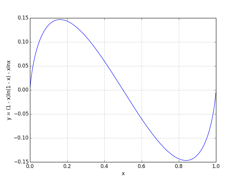
From the above curve, we can verify that $k = \frac{m}{n}\ln 2$ is the only extreme point and it is the minimal point, therefore, it is the minimum point. Therefore, the optimal $k$ is,

$$\begin{equation} k = \frac{m}{n}\ln 2 \end{equation}$$

References